A basic test was run to begin to gain some intuition on the affects of a spatially varying convolution kernels. The goal is to divide the image into sections, apply a different kernel on the different sections, then deconvolve using the correct and/or incorrect kernel. I used Lucy-Richardson deconvolution as well as blind deconvolution.
The Creative Commons Kansas Crops image was taken from Wikipedia because it 1) is similar to an image of interest, 2) varied in texture while having some quality sharpness, 3) maintained similar features throughout.
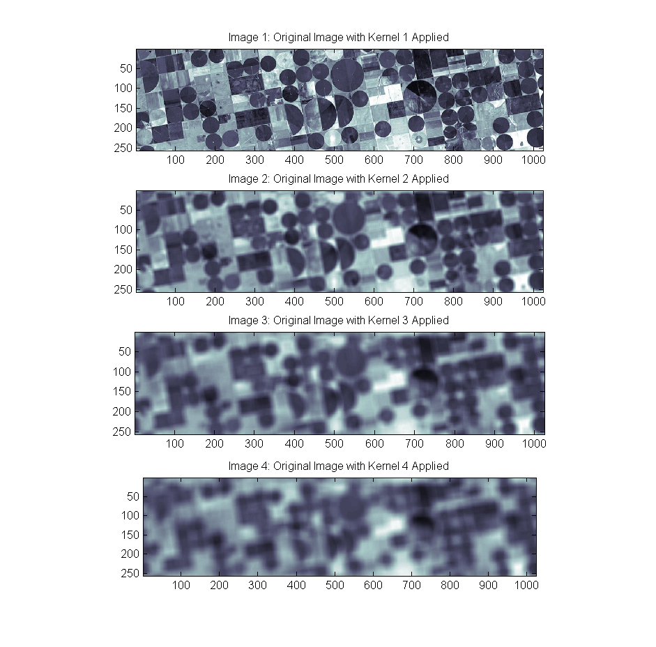
 Box Kernels 1 through 4 were created of size [2, 10, 18, 26] (that’s 2+8*(ind-1)) in order to create a set of blurred images as follows:
 Lucy-Richardson deconvolution was then used to deconvolve the blurred image back into the original by providing it the true kernel used for each image and 100 iterations. While the larger kernels are more challenging, the images to quite well at 100 iterations:
 But what happens when the wrong kernel is used? The answer is: very bad things. Here is an example of the output of running Lucy-Richarddon on the Original Image blurred with kernel 2 but telling Lucy-R to deconvolve using kernel 4:
 To further explore, I created a hybrid image that took 256 x 256 blocks from independent regions of the individual blurred images 1-4 and concatenated them to create a single image with difference independent blurs:
 The Lucy-Richardson Deconv. routine was then run and given each of the for 4 kernels:
 The results are consistent with the individual Image2/Kernel4 combo shown above with the added problem that the transition between the two regions is quite abrupt.
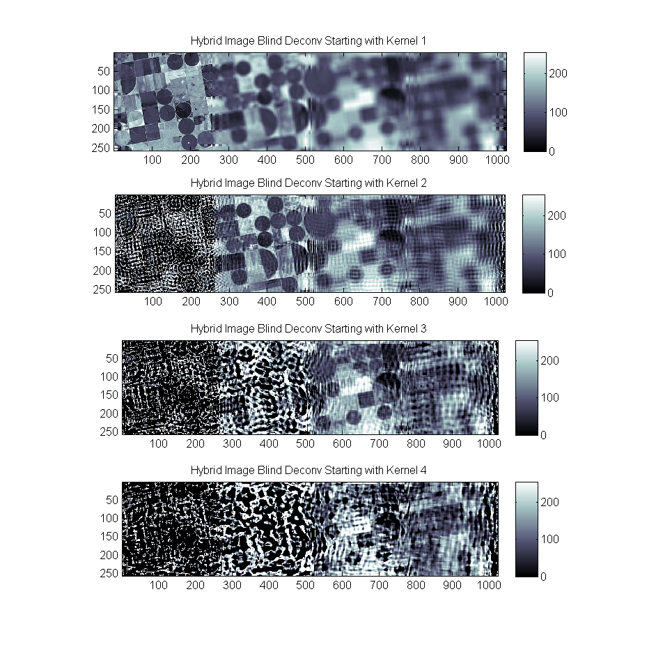
A final test was run showing the results of blind deconvolution on the hybrid image starting with Kernel1 through kernel4 as an initial guess. The results are similar:
As noted, a certain unkindness has been done to the deconvolution in both the Lucy and the Blind case. Since the hybrid was created with abrupt changes from one kernel to the next we introduce a visible discontinuity on the border of the regions. While the transition will always be there this results in significant problems in the frequency domain and causes ringing in spatial domain as well.
Further improvements will be to begin to address the non-homogeneity of the blurring kernel directly as well as consider the transition regions.


One Reply to “Introductory Plots for Deconvolution”